
What are spatial and spatio-temporal modeling?
People experience health outcomes, such as contracting a disease, at different points in time and in different locations. Epidemiologists who want to describe, explain and predict disease occurrence use spatial models to account for location, and spatio-temporal models to account for location and time, along with any known or hypothesized determinants of the disease condition. They present their findings as a map or a sequence of maps predicting the prevalence or incidence of the condition.
Examples of health outcomes that have been modeled in this way include incidence of cholera, traffic accidents, cases of Zika virus and pre-term births, or prevalence of tuberculosis, specific cancers and obesity.
Spatial modeling
Spatial modeling describes investigations which locate observations geographically at a specific time or during a period of time when investigators assume the event is stable. The goal in spatial analysis is to investigate geographic variation in the probability of occurrence of the health outcome.
Spatio-temporal modeling
Spatio-temporal modeling describes studies which record and analyse both the locations and associated times of the observations. In spatio-temporal analysis, the focus is on variation in the average number of incident or prevalent cases in combinations of place and time units over the geographical region and time-period of interest – that is the spatio-temporal intensity of incident or prevalent cases.
Why spatial and spatio-temporal modeling?
An early, and famous example of a spatial point pattern map being used in a public health context is Dr. John Snow’s 1854 map of cholera in Soho, London although a much less celebrated map of cholera in the northern England city of Leeds was produced by Dr. Robert Baker 22 years earlier.
Prevalence mapping
Maps showing the current and historic distribution of a condition are useful to planners when making long-term decisions about where to allocate resources effectively so as to prevent and control disease among populations at risk. For example:
The Environmental and Health Atlas of England and Wales provides interactive maps for 14 health conditions for neighbourhoods (census wards of about 6000 people) in England and Wales. These maps show risks for each census ward relative to the risk in England and Wales of contracting the condition. The risks are based on disease reporting and are age-adjusted and averaged over a period of about 25 years. Health planners or members of the public can assess the relative risk, for example, of lung cancer, breast cancer, heart disease, or still births for their neighbourhoods.
Snake bites are a serious public health problem in Sri Lanka. Ministry officials need to know where to locate treatment centres and distribute anti-venom. It is impossible to describe the incidence simply by analysing hospital records because not all cases present at health facilities. Ediriweera et al. applied spatial statistical modelling to data from a national survey of snake bite incidence to develop maps for the entire island. He identified where snake bites were most likely to occur and where they were least likely to occur.
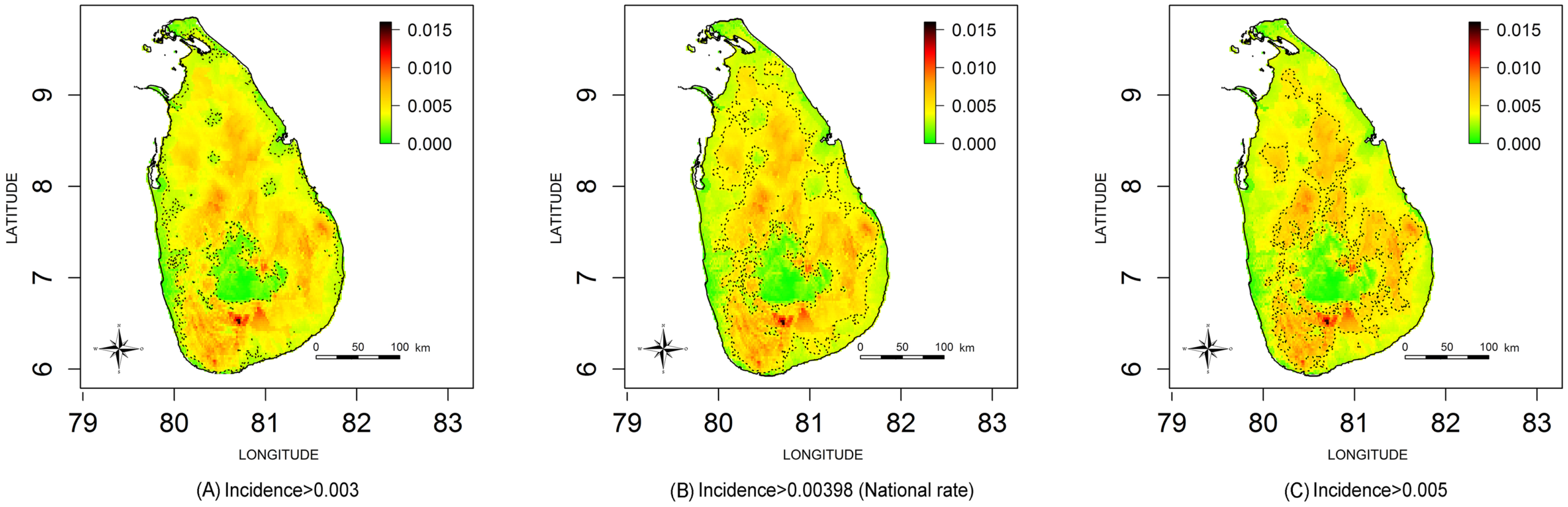
Geographical variation in snake bite incidence per person per year in Sri Lanka September 2011 to August 2012 (Source Ediriweera et al.)
Real time surveillance
Real-time spatio-temporal surveillance can inform a rapid response team about where and when to target prevention and control activities as well as to make longer term plans.
For example, the New York City Department of Health developed a system that uses daily reports of the location and timing of 35 notifiable diseases to automatically detect epidemics. In 2015, the system identified a cluster of community-acquired legionellosis in a specific location three days before health professionals noticed an increase in cases; the cluster of observations expanded and became the largest outbreak in the US.
Types of spatio-temporal study design
Study design depends on the objectives of the study and practical constraints.
Longitudinal design
In a longitudinal design, data are collected repeatedly over time from the same set of sampled locations. This is appropriate when temporal variation in the health outcome dominates spatial variation. A longitudinal design can be cost-effective when setting up a sampling location is expensive but subsequent data-collection is cheap. Longitudinal designs can act as sentinel locations, when the locations may be chosen subjectively, either to be representative of the population at large or, in the case of pollution monitoring for example, to capture extreme cases to monitor compliance with environmental legislation.
Repeated cross-sectional design
In a repeated cross-sectional design, the researcher chooses different sets of locations on each sampling occasion. This sacrifices direct information on changes in the underlying process over time in favour of more complete spatial coverage. For example, to predict stunting in children in Ghana, researchers drew data from four quinquennial national Demographic and Health Surveys each of which used a similar two-stage cluster sampling strategy.
Repeated cross-sectional designs can also be adaptive, meaning that on any sampling occasion, the choice of sampling locations is informed by an analysis of the data collected on earlier occasions. Adaptive repeated cross-sectional designs are particularly suitable for applications in which temporal variation either is dominated by spatial variation or is strongly related to risk factors of interest.
Types of data
Spatially referenced data
Researchers can collect spatially referenced data in at least three different formats, depending on their study design.
Spatial point pattern data-set
The unit of observation is the individual case which the researcher geo-references to a single point in the region being described. For example all persons diagnosed with cholera in the region, each identified by their village address.
Geo-statistical data-set
The unit of observation is a location in the region but the researcher obtains the data only from a sample of the susceptible population. Typically, each location identifies a village community but resource limitations dictate that use only of a sample of villages, rather than a complete census. The data-set consists of the number of cases in each sampled village.
Small-area data-set
The researcher partitions the region into a set of sub-regions. The dataset consists of all cases of cholera in each sub-region. Typically the researcher uses this approach when the health system maintains a register of all cases in the region.
All these formats can be extended in time. For example when an investigator records both the location and time of occurrence of a case during real-time surveillance, they obtain a spatio-temporal point pattern data-set of all cases. When the investigator records cases longitudinally at sampled locations, they obtain a spatio-temporal geostatistical data-set, and similarly with small area data-sets.
Geostatistical data-sets are most commonly obtained for disease mapping and surveillance in low-resource settings where collecting point pattern data is expensive and health registries may not exist to provide small area data.
Sampling and geostatistical data-sets
Without a properly designed sampling scheme, there is a risk that the investigator will sample more accessible communities that do not represent the health experiences of the study-population, that is the study will be biased.
To obtain valid predictions, the sample must be as unbiased spatially and temporally. The sampling schemes below are commonly used to eliminate as much bias as possible.
Probability sampling
To avoid spatial bias the investigator can either selecting gridded locations from a gridded map of the geographic area of interest or use a probability sampling scheme.
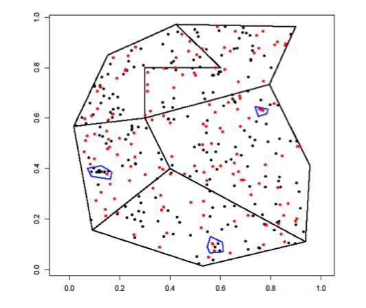
Counter-intuitively, simple random sampling is not recommended. The reason is that this leads to an irregular pattern of sampled locations; for constructing an accurate map, is is preferable to evenly space sampling locations throughout the region of interest. Chipeta et al. explain how this can be achieved without losing the guarantee of unbiasedness by choosing sampling locations at random subject to the constraint that no two sampled location can be separated by less than a specified minimum distance.
Stratified random sampling
Stratified random sampling is a set of simple random samples, one in each of a pre-defined set of sub-regions that form a partition of the region of interest. Chipeta et al.’s method can secure an even coverage of each sub-region without introducing bias. Stratification generally leads to gains in efficiency when contextual knowledge can be used to define the strata . So between-strata variation in the outcome of interest dominates within-stratum variation.
Multi-stage cluster sampling
The investigator divides the region of interest into administrative divisions and randomly selects a number of clusters of households or villages in each division. Cluster sampling designs are typically less efficient statistically than simple or stratified designs with the same total sample size. But this is counterbalanced by their practical convenience.
Opportunistic sampling
To reduce the length and cost of the study, researchers often use opportunistic sampling, in which they collect data at whatever locations are available, for example from presentations at health clinics. The limitations are obvious. the onus is on the investigators to convince themselves and their audience that such a design does not bias their results.
Types of statistical modeling
Analysts use either empirical and mechanistic models although the distinction is not always clear-cut.
- An empirical model can describe and predict the phenomenon of interest. The suitability of this model is determined by its fit to the data and its ability to make useful predictions.
- A mechanistic model seeks to explain why the phenomenon is as it is by incorporating specific, subject-related knowledge.
Mechanistic models are conceptually more appealing than empirical models. This appeal is not cost-free. Adding complexity to a statistical model inevitably results in estimates of its parameters that are less precise, unless additional assumptions that are not easily validated from the available data can be justified by subject-matter knowledge.
We explain here three common applications of empirical models.
For detailed descriptions of the underlying statistical methods, see Gelfand et al.
Prevalence mapping
In prevalence mapping, our goal is to predict the probability that a randomly sampled individual living at a specific location anywhere in the region of interest will be a case. Suppose: the observed number of cases at any one location follows a specific distribution (a binomial distribution); and that these observations are spatially correlated, typically with the value of the correlation between any two observations depending on their spatial separation.
We formulate a generalized linear mixed model to explain the observations in terms of measured explanatory variables and spatial variation, and estimate model parameters using likelihood-based methods.
We then use the model and its parameters to predict the probability of a case occurring at observed and unobserved locations. This resource that explains geostatistical modelling for prevalence and incidence mapping. For example:
Ediriweera et al. counted the number of snakebites reported by households at locations in each sampled district and observed sociodemographic data about the sampled community such as mean age, percentage males, and mean income. They classified each district environmentally, for example by its climatic zone, elevation and land cover. They built a model to explain the distribution of snake bites in terms of these variables. They then estimated its parameters, and predicted the probability of a snake bite occurring in all districts of Sri Lanka. To make predictions in districts that they had not sampled, they used published data on the explanatory variables. for example from the census and from global environmental sources. They presented their findings as incidence of snake bites per person per year and also as levels of snake bite probabilities with contours on a map of Sri Lanka.
Diggle et al. used the same modelling framework to map the geographical variation in Loa loa prevalence in rural communities throughout Cameroon. Strictly, the true prevalence must vary over time. But because infection with Loa loa parasites is both endemic and long-lasting in the absence of any intervention, a purely spatial map remains relevant for some time after it is produced. As well as mapping prevalence, the researchers mapped the probability that prevalence exceeded 20 per cent – or exceedance probabilities as shown in the map below.
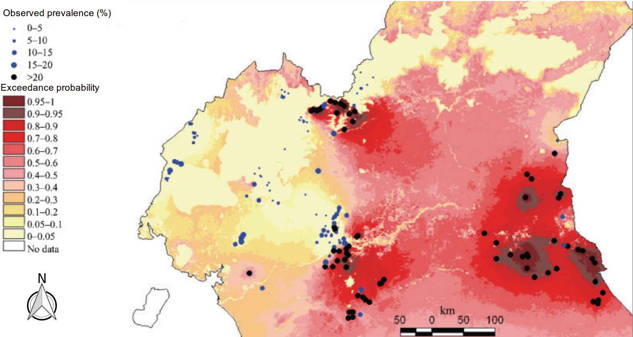
Predictive probability that prevalence of Loaloa in rural communities in Cameroon exceeds 20 per cent. For details, see Diggle et al.
The same type of model can also be used for case-control studies, where the response from each study participant is now one for a case and zero for a control.
For example, to understand the spatial clustering of childhood cancers in Spain, Ramis et al. undertook a case-control study. Cases were children aged zero to fourteen years diagnosed in five Spanish regions for the period 1996-2011 with three major childhood causes of cancer. For the control group, they sampled from the birth registry six controls for each case, matched by year of birth, autonomous region of residence and sex. They geo-coded and validated the addresses of the cases and controls. By comparing the two point patterns, they drew conclusions about variation in risk within each autonomous region while controlling for age and sex effects. Matching by autonomous region meant that they could not compare risks between different autonomous regions.
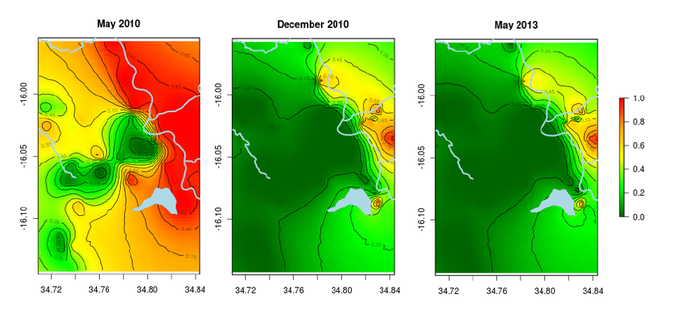
Prevalence mapping over time
When undertaking spatio-temporal analysis of geostatistical data, the goal is to predict
The intensity, or the mean number, of cases per unit area per unit time at a specific location and a specific time over a geographical region of interest.
We use the same approach but associate time with the observations and the explanatory variables, and explain the remaining variation as correlations in both space and time.
The problem with this type of analysis is that computations can be unwieldy. The researcher should keep the model as simple as possible. For example, in some applications it is possible to explain annual variation in the outcome of interest by known seasonally varying risk-factors. So that inclusion of appropriate seasonal explanatory variables may allow us to drop time from the unexplained variation.
Models and inferential algorithms for spatio-temporal mapping are a continuing topic of statistical research, see, for example, Cressie and Wikle or Shaddick and Zidek.
Real-time surveillance
A surveillance study sets out to understand the current status of a dynamically changing phenomenon. The data in this case are usually in the form of a spatio-temporal point pattern covering a defined geographic region. We use the same methods as above but use custom-made software to constantly update the model by entering data in real-time. A resource that explains spatio-temporal statistical methods for real-time surveillance is Diggle et al.
For example, around 2000, some of the authors worked with the United Kingdom’s Public Health Laboratory Service in an English county. They aimed to identify anomalous incidence patterns of symptoms typically associated with foodborne disease. They fed daily data from a 24-hour phone-in helpline into bespoke software. They then computed, for each location, the probability that the underlying incidence on that day exceeded expectation by a factor of two or more. The local Laboratory Service presented the updated map of exceedance probabilities on a website by the start of the next working day.
In low resource settings, reliable automated data feeds are less likely to be available. In their absence, the same underlying principles nevertheless hold. The over-riding aim is to update results in response to new data in as timely a manner as possible. If real-time data-acquisition means collecting new data weekly or monthly, rather than daily, it may also be possible to build an adaptive design element onto a surveillance system. This could make the best use of the limited resources available for the next data collection; see Chipeta et al.
Presentation of the findings as maps
Our preference is to map the predictive probability that prevalence exceeds a specified value, ideally one that relates to an operational, policy-based threshold. These are percentile maps.
An alternative would be to use a series of predictive quantile maps. Rather than map the predictive probability at each location of exceeding a fixed threshold, we do the converse. We map the value at each location that is exceeded with a fixed probability.
From the latter perspective, a pair of maps corresponding to, say the 0.05 and 0.95 points in the predictive distribution at each location would represent pointwise 90% credible intervals for the true prevalence. For a complete picture, this approach requires the analyst to produce a series of maps at different percentile or quantile thresholds. Ideally these are a dynamic image with one or more sliders to control the display.
Computation
The methods for analysing spatial and spatio-temporal data are freely available via packages written for the R open-source statistical computing environment. The R environment also offers packages that mimic many GIS features; alternatively, the user can conduct their statistical analysis in R and pass the output to their preferred GIS.
GIS software can include implementations of some quite sophisticated spatial statistical methods. The user should use caution in adopting the software unless they are an experienced statistician. These implementations often make poor, sometimes automated, choices for the underlying model parameters. More seriously, the applications do not encourage the user to question the validity of the model assumptions.
Challenges
Not every health research or policy agency has an in-house team of professional statisticians. It is important o alleviate the shortage of statisticians in low- and middle-income countries. A long-term strategy of international collaboration can build in-country capacity in statistics.
Maintaining complex real-time surveillance systems can be challenging. However, the deep penetration of mobile phone technology throughout the world makes it possible for field workers in remote locations to upload routine clinical data. They can transfer these data to a central location for sophisticated, computationally intensive processing. They can then feed the results back to local users in real-time.
The quality of data and databases is critical. No amount of sophisticated statistical modelling can produce reliable evidence from unreliable data. But statistical modelling can extract greater value from geographically sparse health outcome data by linking them with freely available geographically dense data on social and natural environmental factors.
Contents
Additional resources
The complete chapter on which we based this page:

Diggle P., Giorgi E., Chipeta M., Macfarlane S.B. (2019) Tracking Health Outcomes in Space and Time: Spatial and Spatio-temporal Methods. In: Macfarlane S., AbouZahr C. (eds) The Palgrave Handbook of Global Health Data Methods for Policy and Practice. Palgrave Macmillan, London.
COVID-19 resources
Jia et al. Population flow drives spatio-temporal distribution of COVID-19 in China
Briz-Redón A, Serrano-Aroca A. A spatio-temporal analysis for exploring the effect of temperature on COVID-19 early evolution in Spain
Adekunle A. et al. Modelling spatial variations of coronavirus disease (COVID-19) in Africa
Latest COVID-19 publicationts ⇒
Other resources
Mateu, J, Muller WG. Spatio-temporal design: advances in efficient data acquisition.
Gelfand AE, Diggle P, Guttorp P, Fuentes M. Handbook of spatial statistics.
Diggle PJ, Giorgi E. Model-based geostatistics for prevalence mapping in low-resource settings.
Wikle C, Cressie NA. Statistics for spatio-temporal data.
Shaddick G, Zidek JV. Spatio-temporal methods in environmental epidemiology
Latest publications ⇒